What does 100 percent busy mean?
How should utilization, response time, and service time really be calculated?
August 1999
|
|
What does 100 percent busy mean?How should utilization, response time, and service time really be calculated? |
August 1999 |
Complex systems can be 100 percent busy, but still have a lot of spare capacity. Adrian looks at this apparent paradox, explains what the real meaning of the term utilization is, and gives advice on how to use and interpret utilization values. (2,200 words)
|
Mail this article to a friend |
![]() : Some of my disks get really slow when they are nearly 100 percent busy; however, when I see a striped volume or hardware RAID unit at high utilization levels, it still seems to respond quickly. Why is this? Do the old rules about high utilization still apply?
: Some of my disks get really slow when they are nearly 100 percent busy; however, when I see a striped volume or hardware RAID unit at high utilization levels, it still seems to respond quickly. Why is this? Do the old rules about high utilization still apply?
![]() : This occurs because more complex systems don't obey the same rules as simple systems when it comes to response time, throughput, and utilization. Even the simple systems aren't so simple. I'll begin our examination of this phenomenon by looking at a single disk, and then move on to combinations.
: This occurs because more complex systems don't obey the same rules as simple systems when it comes to response time, throughput, and utilization. Even the simple systems aren't so simple. I'll begin our examination of this phenomenon by looking at a single disk, and then move on to combinations.
Part of this answer is based on my September 1997 Performance Q&A column. The information from the column was updated and included in my book as of April 1998, and has been further updated for inclusion in Sun BluePrints for Resource Management. Written by several members of our group at Sun, this book will be published this summer (see Resources for more information on both the book and the column). I've added much more explanation and several examples here.
Measurements on a single disk
In an old-style, single-disk model, the device driver maintains a queue of waiting requests that are serviced one at a time by the disk. The terms utilization, service time, wait time, throughput, and wait queue length have well-defined meanings in this scenario; and, for this sort of basic system, the setup is so simple that a very basic queuing model fits it well.
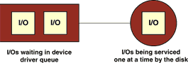
Figure 1. The simple disk model |
Over time, disk technology has moved on. Nowadays, a standard disk
is SCSI-based and has an embedded controller. The disk drive
contains a small microprocessor and about 1 MB of RAM. It
can typically handle up to 64 outstanding requests via SCSI
tagged-command queuing. The system uses an SCSI host bus adaptor to talk to the disk. In large systems, there is yet another level of intelligence and buffering in a hardware RAID controller. However, the iostat utility is still built around the simple disk model above, and its use of terminology still assumes a single disk that can only handle a single request at a time. In addition, iostat uses the same reporting mechanism for client-side NFS mount points and complex disk volumes set up using Solstice DiskSuite or Veritas Volume Manager.
In the old days, if the device driver sent a request to the disk,
the disk would do nothing else until it completed the request. The
time this process took was the service time, and the average service time was a physical property of the disk itself. Disks that spun and sought
faster had lower (and thus better) service times. With today's systems, if
the device driver issues a request, that request is queued
internally by the RAID controller and the disk drive, and several
more requests can be sent before a response to the first comes back. The
service time, as measured by the device driver, varies according to
the load level and queue length, and is not directly comparable to
the old-style service time of a simple disk drive. The response time
is defined as the total waiting time in the queue plus the service
time. Unfortunately, as I've mentioned before, iostat reports
response time but labels it svc_t. We'll see later how to calculate
the actual service time for a disk.
As soon as a device has one request in its internal queue, it becomes busy, and the proportion of the time that it is busy is the utilization. If there is always a request waiting, then the device is 100 percent busy. Because a single disk can only complete one I/O request at a time, it saturates at 100 percent busy. If the device has a large number of requests, and it is intelligent enough to reorder them, it may reduce the average service time and increase the throughput as more load is applied, even though it is already at 100 percent utilization.
The diagram below shows how a busy disk can operate more efficiently than a lightly loaded disk. In practice, the main difference you would see would be a lower service time for the busy disk, albeit with a higher average response time. This is because all the requests are present in the queue at the start, so the response time for the last request includes the time spent waiting for every other request to complete. In the lightly loaded case, each request is serviced as it is made, so there is no waiting, and response time is the same as the service time. If you hear your disk rattling on a desktop system when you start an application, it's because the head is seeking back and forth, as shown in the first case. Unfortunately, starting an application tends to generate a single thread of page-in disk reads. Each such read is not issued until the previous one is completed, so you end up with a fairly busy disk with only one request in the queue -- and it can't be optimized. If the disk is on a busy server instead, there are numerous accesses coming in parallel from different transactions and different users, so you will get a full queue and more efficient disk usage overall.
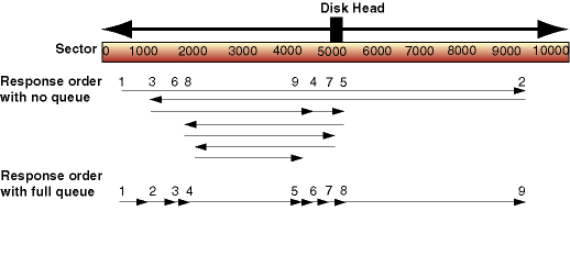
Figure 2. Disk head movements for a request sequence |
Solaris disk instrumentation
The instrumentation provided in the Solaris operating environment
takes account of this change by taking a request's waiting period and breaking it up into two separately measured queues. One queue, called the wait queue, is in the device driver; the other, called the active queue, is in the device itself. A read
or write command is issued to the device driver and sits in the wait
queue until the SCSI bus and disk are both ready. When the command
is sent to the disk device, it moves to the active queue until the
disk sends its response. The problem with iostat is that it tries to
report the new measurements using some of the original terminology.
The wait service time is actually the time spent in the wait
queue. This isn't the correct definition of service time, in any case,
and the word wait is being used to mean two different things.
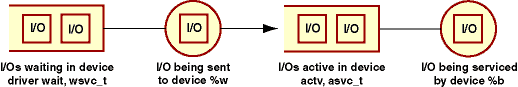
Figure 3. Two-stage disk model used by Solaris 2 |
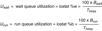
Utilization (U) is defined as the busy time (B) as a percentage of the total time (T) as shown below:
|
iostat prints out and calls svc_t. This is the real thing! It can be calculated as the busy time (B) divided
by the number of accesses that completed, or alternatively as the
utilization (U) divided by the throughput (X):
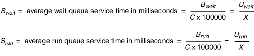
|
iostat output, you need to divide the utilization by the total number of reads and writes, as we see here.
 % iostat -xn
...
                              extended device statistics
  r/s  w/s   kr/s   kw/s wait actv wsvc_t asvc_t   %w   %b device
 21.9 63.5 1159.1 2662.9  0.0  2.7    0.0   31.8   0    93 c3t15d0
In this case U = 93% = 0.93, and throughput X = r/s + w/s = 21.9 + 63.5 = 85.4; so, service time S = U/X = 0.011 = 11 milliseconds (ms), while the reported response time R = 31.8 ms. The queue length is reported as 2.7, so this makes sense, as each request has to wait in the queue for several other requests to be serviced.
Using the SE Toolkit, a modified version of iostat written in SE
prints out the response time and the service time data, using the
format shown below.
 % se siostat.se 10
03:42:50  ------throughput------ -----wait queue----- ----active queue----
disk      r/s  w/s   Kr/s   Kw/s qlen res_t svc_t  %ut qlen res_t svc_t  %ut
c0t2d0s0  0.0  0.2    0.0    1.2 0.00  0.02  0.02    0 0.00 22.87 22.87   0
03:43:00  ------throughput------ -----wait queue----- ----active queue----
disk      r/s  w/s   Kr/s   Kw/s qlen res_t svc_t  %ut qlen res_t svc_t  %ut
c0t2d0s0  0.0  3.2    0.0   23.1 0.00  0.01  0.01    0 0.72 225.45 16.20   5
We can get the number that iostat calls service time. It's defined as the queue length (Q, shown by iostat with the headings wait and actv) divided by the throughput; but it's actually the residence or response time and includes all queuing effects:
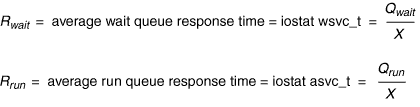
|
iostat example, R = Q / X = 2.7 / 85.4 =
0.0316 = 31.6 ms, which is close enough to what iostat reports. The
difference between 31.6 and 31.8 is due to rounding
errors in the reported values of 2.7 and 85.4. Using full precision,
the result is identical to what iostat calculates as the response
time.
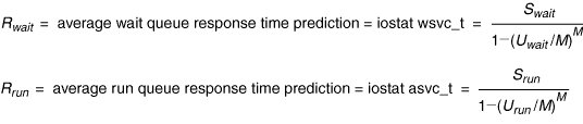
Another way to express response time is in terms of service time and utilization. This method uses a theoretical model of response time that assumes that, as you approach 100 percent utilization with a constant service time, the response time increases to infinity:
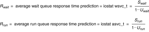
|
|
|
|
|
|
Complex resource utilization characteristics
One important characteristic of complex I/O subsystems is that the utilization measure can be confusing. When a simple system reaches 100 percent busy, it has also reached its maximum throughput. This is because only one thing is being processed at a time in the I/O device. When the device being monitored is an NFS server, a hardware RAID disk subsystem, or a striped volume, the situation is clearly much more complex. All of these can process many requests in parallel.
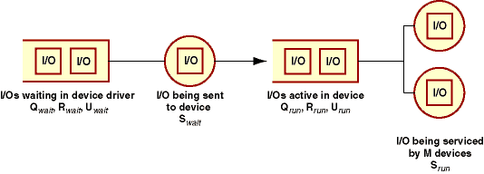
Figure 4. Complex I/O device queue model |
As long as a single I/O is being serviced at all times, the utilization is reported as 100 percent, which makes sense because it means that the pool of devices is always busy doing something. However, there is enough capacity for additional I/Os to be serviced in parallel. Compared to a simple device, the service time for each I/O is the same, but the queue is being drained more quickly; thus, the average queue length and response time are less, and the peak throughput is greater. In effect, the load on each disk is divided by the number of disks; therefore, the true utilization of the striped disk volume is actually above 100 percent. You can see how this arises from the alternative definition of utilization as the throughput multiplied by the service time.
With only one request being serviced at a time, the busy time is the time it takes to service one request multiplied by the number of requests. If several requests can be serviced at once, the calculated utilization goes above 100 percent, because more than one thing can be done at a time! A four-way stripe, with each individual disk 100 percent busy, will have the same service time as one disk, but four times the throughput, and thus should really report up to 400 percent utilization.
The approximated model for response time in this case changes so that response time stays lower for a longer period of time; but it still heads for infinity when the underlying devices each reach 100 percent utilization.
|
Wrap up
So the real answer to our initial question is that the model of disk behavior and performance that is embodied by the iostat report is too simple to cope with the reality of a complex underlying disk subsystem. We
stay with the old report to be consistent and to offer users
familiar data, but in reality, a much more sophisticated approach is
required. I'm working (slowly) on figuring out how to monitor and
report on complex devices like this.
![]()
|
|
Resources
virtual_adrian.se rule:
About the author
![]() Adrian
Cockcroft joined Sun Microsystems in 1988, and currently works as a
performance specialist for Sun's Computer Systems Division. He
wrote Sun
Performance and Tuning: SPARC and Solaris and Sun
Performance and Tuning: Java and the Internet, both published
by Sun Microsystems Press
Books.
Adrian
Cockcroft joined Sun Microsystems in 1988, and currently works as a
performance specialist for Sun's Computer Systems Division. He
wrote Sun
Performance and Tuning: SPARC and Solaris and Sun
Performance and Tuning: Java and the Internet, both published
by Sun Microsystems Press
Books.
|
|
|
|
If you have technical problems with this magazine, contact webmaster@sunworld.com
URL: http://www.sunworld.com/swol-08-1999/swol-08-perf.html
Last modified: