Click on our Sponsors to help Support SunWorld

Getting to know the Solaris filesystem, Part 2

What factors influence filesystem performance?

By Richard McDougall

June 1999

Abstract

Last month Richard walked you though some of the major features of three common filesystems for Solaris: the Solaris UFS filesystem, Veritas's VxFS filesystem, and LSC's QFS filesystem. This month he looks at some of the factors, including filesystem configuration options, that affect filesystem performance. (7,300 words)

Mail this
article to
a friend

ilesystem performance is a major component of overall system performance and is heavily dependent on the nature of the application generating the load. To achieve optimal performance, the underlying filesystem configuration must be balanced to match the application characteristics.

If you're a developer, you might already have a good idea of how your application is reading or writing though the filesystem; if you're an administrator of an application, however, you might need to spend some time analyzing the application in order to understand the type of I/O profile being presented to the filesystem.

Once we have a good understanding of the application, we can try to optimize the filesystem configuration to make the most efficient use of the underlying storage device. Our objective is to

Reduce the number of I/Os to the underlying device(s) where possible
Group smaller I/Os together into larger I/Os where possible
Optimize the seek pattern to reduce the amount of time spent waiting for disk seeks
Cache as much as data as we realistically can to reduce physical I/Os

We'll only touch on filesystem caching this month, leaving the bulk of Solaris caching implementation for next month. If you need to brush up on the basics of Solaris filesystems before reading this article, please refer to Part 1 of this series.

Understanding the workload profile
Before we can configure a filesystem, we need to understand the workload characteristics that are going to use the filesystem. We begin by looking at a simple breakdown of application workload profiles. From there, we can determine a given application's profile type by tracing the application.

The important characteristics of the workload profile can be grouped into five categories, which are shown in Table 1.

Characteristic

Values

Description

File access profile

Data or attribute intensive?

Does the application read, write, create, and delete many small files or does it just read and write within existing files?

Access pattern Random, sequential, or strided? Are the reads and writes random or sequentially ordered?

Bandwidth

Megabytes per second

What is the bandwidth requirement of the application? What are the average and peak rates of data that is read from or written to the filesystem from the application?

I/O size

Bytes

What is the most common I/O size requested? Does this match the block size of the filesystem?

Latency sensitive?

Milliseconds

Is the application sensitive to read and -- especially -- write latency?

Characteristic	Values	Description
File access profile	Data or attribute intensive?	Does the application read, write, create, and delete many small files or does it just read and write within existing files?
Access pattern	Random, sequential, or strided?	Are the reads and writes random or sequentially ordered?
Bandwidth	Megabytes per second	What is the bandwidth requirement of the application? What are the average and peak rates of data that is read from or written to the filesystem from the application?
I/O size	Bytes	What is the most common I/O size requested? Does this match the block size of the filesystem?
Latency sensitive?	Milliseconds	Is the application sensitive to read and -- especially -- write latency?

Table 1. Examples of workload characteristics

Now let's look a bit more closely into those five workload characteristics.

Data or attribute intensive
A data-intensive application is one that shifts a lot of data around without creating or deleting many files; an attribute-intensive application is one that creates and deletes a lot of files and only reads and writes small amounts of data in each. An example of a data-intensive workload is a scientific batch program that creates 20-GB files; an example of an attribute-intensive workload is an office automation fileserver that creates, deletes, and stores hundreds of small files, each less than 1 MB in size.

Access patterns
The access pattern of an application has a lot to do with the amount of optimization it will allow. An application can read or write though a file either sequentially or in a random order. Sequential workloads are the easiest to tune because we can group the I/Os and optimize how we issue them to the underlying storage device.

Another type of access pattern is strided access; this is typically found in scientific applications. Strided workloads are sequential in small groups (perhaps 1 MB at a time), after which they seek within the file to another small sequential group. Strided workloads can sometimes read multiple 8-KB blocks at a time before they seek to a new location, making some sequential tuning valid (e.g., read ahead and cluster sizes). But they have caching demands similar to those of random workloads.

Bandwidth
The bandwidth of an application characterizes the amount of data it is shifting to and from its files. In many cases, bandwidth is most useful for capacity-planning the underlying storage devices, but there are also some important caching characteristics that are affected by the amount of bandwidth the application uses.

I/O size
The size of each I/O has a large impact on how the filesystem should be configured. I/O devices generally are much less efficient with smaller I/Os, and we can use the filesystem to group small adjacent I/Os into larger transfers to the storage devices. For random workload patterns, the I/O size has some strong interactions with the block size of the file system.

Latency sensitive
A latency sensitive application is one that is very sensitive to the amount of time taken for each I/O. For example, a database is very sensitive to the amount of time taken to write to its log file. This type of application can really benefit from well-planned caching strategies.

Data-intensive sequential workloads
Sequential workloads are those that perform repetitive I/Os in ascending or descending order, reading or writing sequential file blocks. We typically see sequential patterns when we shift large amounts of data around, like when we copy a file, read a large portion of a file, or write a large portion of a file.

We can use the truss command to investigate the nature of an application's access pattern by looking at the read, write, and lseek system calls. Below, we use the truss command to trace the system calls generated by our application, processid 20432.

# truss -p 20432

read(3, "\0\0\0\0\0\0\0\0\0\0\0\0".., 512)      = 512
read(3, "\0\0\0\0\0\0\0\0\0\0\0\0".., 512)      = 512
read(3, "\0\0\0\0\0\0\0\0\0\0\0\0".., 512)      = 512
read(3, "\0\0\0\0\0\0\0\0\0\0\0\0".., 512)      = 512
read(3, "\0\0\0\0\0\0\0\0\0\0\0\0".., 512)      = 512
read(3, "\0\0\0\0\0\0\0\0\0\0\0\0".., 512)      = 512
read(3, "\0\0\0\0\0\0\0\0\0\0\0\0".., 512)      = 512

We use the arguments from the read system call to determine that the application is reading 512-byte blocks; and because there are no lseek system calls in between each read we can deduce that the application is reading sequentially. When the application requests the first read, the filesystem reads in the first filesystem block for the file, and an 8-KB chunk will be read in. This operation requires a physical disk read, which takes a few milliseconds. The second 512-byte read will simply read the next 512 bytes from the 8-KB filesystem block that is still in memory. This only takes a few hundred microseconds. We only see one physical disk read for each 8 KB worth of data.

This is a major benefit to the performance on the application because each disk I/O takes a few milliseconds. If we were to wait for a disk I/O every 512 bytes, the application would spend most of its time waiting for the disk. Reading the physical disk in 8-KB blocks means that the application only needs to wait for a disk I/O every 16 reads rather than every read, reducing the amount of time spent waiting for I/O.

Read ahead helps sequential performance
Waiting for a disk I/O every 16 512-byte reads is still terribly inefficient; we might only spend a few hundred microseconds processing these 512-byte blocks, yet we can easily spend 10 milliseconds waiting for the next 8-KB block to come from disk. To put this in perspective, this is comparable to catching a bus to travel 10 minutes down the road, deboarding, then waiting 6 hours for the next bus to take us another 10 minutes down the road.

Filesystems are smart enough to be able to work around this problem. Because the access pattern is repeating, the filesystem can predict that it is very likely the next block will be read, given the sequential order of the reads. Most filesystems implement an algorithm that does this, commonly known as the read ahead algorithm. The read ahead algorithm detects that a file is being read sequentially by looking at the current block being requested and comparing it to the last block that was requested. If they're adjacent, the filesystem can initiate a read for the next few blocks as it reads the current block. There's no need to stop and wait for the next block because it has already been read. This is analogous to phoning ahead and booking the next bus, so that when we get off the bus the next one will already be waiting for us and we won't need to wait. The only thing we need worry about now is initiating the read ahead algorithm for enough blocks at a time so that we rarely have to catch up and wait for a physical disk I/O.

The actual algorithms used in each filesystem type vary, but they all follow the same principles; they look at the recent access patterns and decide to read ahead a number of blocks in advance. The number of blocks read ahead is usually configurable, and often the defaults aren't big enough to provide optimal performance.

UFS filesystem read ahead
The UFS filesystem decides when to implement read ahead by keeping track of the last read operation; if the last read and the current read are sequential, a read ahead of the next sequential series of filesystem blocks is initiated. The following criteria must be met to engage UFS read ahead:

The last filesystem read must be sequential with the current one
There must be only one concurrent reader of the file (reads from other processes will break the sequential access pattern for the file)
The blocks of the file being read must be sequentially layered out on the disk
The file must be being read or written via the read and write system calls; memory-mapped files do not use the UFS read ahead

The UFS filesystem uses the notion of cluster size to describe the amount of blocks that are read ahead in advance. This defaults to 7 8-KB blocks (56 KB) in Solaris versions up to Solaris 2.6 (56 KB was the maximum DMA size on ancient I/O bus systems). In Solaris 2.6, the default changed to the maximum size transfer supported by the underlying device, which defaults to 16 8-KB blocks (128 KB) on most storage devices.

The default values for read ahead are often inappropriate and must be set larger to allow optimal read rates. The size of the read ahead cluster should be set very large for high-performance sequential access to take advantage of modern I/O systems. Modern I/O systems are capable of very large bandwidth, but the cost for each I/O is still considerable, and as a result we want to choose as large a cluster size as is possible to minimize the amount of individual I/Os.

We can observe the default behavior of our 512-byte read example by looking at the average size of the I/Os reported for the underlying storage device:

# iostat -x 5

device    r/s  w/s   kr/s   kw/s wait actv  svc_t  %w  %b 
fd0       0.0  0.0    0.0    0.0  0.0  0.0    0.0   0   0 
sd6       0.0  0.0    0.0    0.0  0.0  0.0    0.0   0   0 
ssd11     0.0  0.0    0.0    0.0  0.0  0.0    0.0   0   0 
ssd12     0.0  0.0    0.0    0.0  0.0  0.0    0.0   0   0 
ssd13     49.0 0.0 6272.0    0.0  0.0  3.7   73.7   0  93 
ssd15     0.0  0.0    0.0    0.0  0.0  0.0    0.0   0   0 
ssd16     0.0  0.0    0.0    0.0  0.0  0.0    0.0   0   0 
ssd17     0.0  0.0    0.0    0.0  0.0  0.0    0.0   0   0

The iostat command shows us that we are issuing 49 read operations per second to the disk ssd113, and averaging 6,272 KBps from the disk. If we divide the transfer rate by the number of I/Os per second, we derive that the average transfer size is 128 KB. This confirms that the default 128-KB cluster size is grouping the 512-byte read requests into 128-KB groups.

We can look at the cluster size of a UFS filesystem by using the mkfs command with the -m option to reveal the current filesystem parameters, as shown below in Figure 1. The cluster size or read ahead size is shown by the maxcontig parameter.

# mkfs -m /dev/rdsk/c1t2d3s0
mkfs -F ufs -o nsect=80,ntrack=19,bsize=8192,fragsize=1024,
cgsize=32,free=4,rps=90,nbpi=4136,opt=t,apc=0,gap=0,nrpos=8,
maxcontig=16 /dev/rdsk/c1t2d3s0 3105360

UFS

VxFS

Figure 1. Sample cluster size of a UFS filesystem as revealed by mkfs -m

For this filesystem, we can see that the cluster size is 16 blocks of 8,192 bytes, or 128 KB. As an alternative, you can use the fstyp -v command on some filesystems, as shown in Figure 2.

# fstyp -v /dev/dsk/c1t4d0s2 ufsmagic 11954 format dynamic time Sun May 23 16:16:40 1999 sblkno 16 cblkno 24 iblkno 32 dblkno 400 sbsize 2048 cgsize 5120 cgoffset 40 cgmask 0xffffffe0 ncg 86 size 2077080 blocks 2044038 bsize 8192 shift 13 mask 0xffffe000 fsize 1024 shift 10 mask 0xfffffc00 frag 8 shift 3 fsbtodb 1 minfree 3% maxbpg 2048 optim time maxcontig 16 rotdelay 0ms rps 90 csaddr 400 cssize 2048 shift 9 mask 0xfffffe00 ntrak 19 nsect 80 spc 1520 ncyl 2733 cpg 32 bpg 3040 fpg 24320 ipg 2944 nindir 2048 inopb 64 nspf 2 nbfree 190695 ndir 5902 nifree 247279 nffree 304 cgrotor 31 fmod 0 ronly 0 fs_reclaim is not set filesystem state is valid, fsclean is 2

UFS

Figure 2. Sample cluster size in a UFS filesystem as revealed by fstyp -v

Calculating read ahead cluster sizes
As a general rule of thumb, I like to ensure that no device has to do more than 200 I/O operations per second to achieve maximum bandwidth. This rule allows us to pick the optimal cluster size for filesystem read ahead. By keeping the number of I/O operations per second low, we also save a lot of host CPU time because the operating system doesn't need to issue as many SCSI requests. This rule provides valid cluster sizes for all the storage devices I've come across to date.

The previous example (shown with iostat) was able to achieve the maximum bandwidth achievable by this 7,200-RPM, 4-GB disk -- needing only 49 I/O operations per second. Today's 10,000-RPM disk drives are capable of transfer rates up to 20 MBps, and also work well with the default cluster size of 128 KB. Some of the more advanced storage devices, such as hardware RAID controllers or software RAID stripes with many disks, are capable of much higher transfer rates. You'll typically see 50 MBps to 100 MBps from most modern storage devices. When we put a filesystem on top of one of these devices, we must use different values for the cluster sizes to achieve efficient read ahead.

Using the 200-operations-per-second rule, a Sun A5200 fiber storage array that can do 100 MBps would need a 512-KB cluster size to allow us to saturate the device with 200 I/O operations per second.

Setting cluster sizes for RAID volumes
There are two other important things we must consider before we leap in and configure our cluster size to larger than 128 KB. The first is that the SCSI drivers in Solaris limit the maximum size of an SCSI transfer to 128 KB by default. Even if we configure the filesystem to issue 512-KB requests, the SCSI drivers will break the requests into smaller 128-KB chunks. The same limit applies with volume managers like Solstice Disk Suite and Veritas Volume Manager. Whenever we use a device that requires us to use larger cluster sizes, we need to set the SCSI and volume manager parameters in the /etc/system configuration file to allow bigger transfers. The following changes in /etc/systemprovide the necessary configuration for larger cluster sizes.

*
* Allow larger SCSI I/O transfers, parameter is bytes
*
set maxphys = 1048576

*
* Allow larger DiskSuite I/O transfers, parameter is bytes
*
set md_maxphys = 1048576

*
* Allow larger VxVM I/O transfers, parameter is 512 byte units
*
set vxio:vol_maxio = 2048

The second thing we need to consider is that RAID devices and volumes often consist of several physical devices that are arranged as one larger volume, and we need to pay attention to what happens to these large I/O requests when they arrive at the RAID volume. For example, a simple RAID level 0 stripe can be constructed from seven disks in a Sun A5200 storage subsystem. I/Os are then interlaced across each of the seven devices according to the interlace size or stripe size. (For a linked list of previous and current SunWorld articles about RAID devices and volumes, see this article's Resources section.)

By interlacing I/O operations across separate devices, we can potentially break up the I/O that comes from the filesystem into several requests that can occur in parallel. Consider a single 512-KB read request that comes from our filesystem: When it arrives at a RAID volume that is configured with a 128-KB interlace size, it will be broken into four, rather than seven, separate 128-KB requests.

Because we have seven separate disk devices in our RAID volume, we have the ability to perform seven I/O operations in parallel. Ideally, we should also have the filesystem issue a request that will initiate I/Os on all seven devices at once. So that it will split into exactly seven components when it is broken up, we must initiate an I/O the size of the entire stripe width of the RAID volume. This requires us to issue I/Os that are 7 KB multiplied by 128 KB, or 896 KB each. In order to do this, we must set the cluster size to 896 KB.

RAID level 5 is similar, but we must remember that we only have an effective space of n - 1 devices. Therefore, an eight-way RAID level 5 stripe will have the same stripe width and cluster size as a seven-way RAID 0 stripe. The guidelines for cluster sizes on RAID 5 devices are as follows:

RAID level 0 striping: Cluster size is equal to number of stripe members multiplied by the interlace size
RAID level 1 mirroring: Cluster size is the same as for a single disk
RAID level 1 + 0 striping + mirroring: Cluster size is equal to number of stripe members per mirror multiplied by the interlace size

We can either set the cluster size at the time we create the filesystem using the newfs command, or after the fact by using the tunefs command. To create a filesystem in UFS with an 896-KB cluster size, we would use the newfs command with the -C option, as follows:

# newfs -C 112 /dev/md/dsk/d20

We can change the cluster size after the filesystem has been created using the tunefs command:

# tunefs -a 112 /dev/md/dsk/d20

Limitations of UFS read ahead
It is important to note that the UFS read ahead algorithms do not differentiate between multiple readers; thus, two processes reading the same file will break the read ahead algorithms.

VxFS filesystem read ahead
The Veritas VxFS filesystem also implements read ahead, but VxFS uses a different mechanism for setting the read ahead size.

The read ahead size for VxFS is set automatically when using the Veritas Volume Manager (VVM) at mount time. The mount command queries the VVM and sets the read ahead options to suit the underlying volume. Alternatively, the options can be set at mount time by command-line options or by entries in the /etc/vx/tunefstab.

The VxFS filesystem uses a parameter, read_pref_io, in conjunction with the read_nstream parameter to determine how much data to read ahead. The default read ahead is 64 KB. The parameter read_nstream reflects the desired number of parallel read requests, each with a size given by read_pref_io, to have outstanding at one time. The filesystem uses the product of read_nstream multiplied by read_pref_io to determine its read ahead size. The default value for read_nstream is 1.

The example below sets the read ahead size to 896 KB using the vxtunefs command:

# mount -F vxfs /dev/dsk/c0t3d0s7 /mnt

# vxtunefs -o read_pref_io=917504 /mnt

QFS filesystem read ahead
LSC Inc.'s QFS filesystem implements read ahead in a similar manner and also uses the maxcontig parameter to reflect the number of blocks per cluster for read ahead. The QFS filesystem maxcontig parameter must be set at mount time, by using the -o maxcontig option:

# mount -o maxcontig=112 samfs1

Storage device read ahead
Modern I/O systems often have some intelligence in the storage device, making prefetching possible at this level. For example, the A3500 storage controller has options to control the read ahead size performed at the controller level which should be aligned with the cluster size of the filesystem.

The Sun A3500 storage controller has comprehensive read ahead options in hardware. For more information on this, see the A3500 user's guide.

Read ahead with memory-mapped files
Memory-mapped files invoke different read ahead algorithms because they bypass the read logic of the filesystem. Sequential access though a memory-mapped file is either detected or forced using MAV_SEQUENTIAL in the memory segment driver (seg_vn) that implements mapped files. Read ahead doesn't use the filesystem cluster size -- it's fixed at 64 KB.

Filesystem write behind
If we were to write each I/O synchronously, we would have to wait a long time in between processing for each write operation to complete. In fact, we would likely spend most of our execution time waiting for the I/Os to complete. Unix employs a far more efficient method to process writes. It passes the writes over to the operating system, which allows the application to continue processing. This method of delayed asynchronous writes is the Unix filesystem's default method to write data blocks; synchronous writes are used only when a special file option is set.

Delayed asynchronous writes allow the application to continue to process without having to wait for each I/O, and also allow the operating system to delay the writes long enough to group together adjacent writes. When we're writing sequentially, this allows us to issue a few large writes, rather than several small writes. As we discussed earlier, it's far more efficient to execute a few large writes than many small writes.

UFS filesystem write behind
The UFS filesystem uses the same cluster size parameter, maxcontig, to control how many writes are grouped together before a physical write is performed. The guidelines used for read ahead should also be applied to write behind. Again, if a RAID device is used, care should be taken to align the cluster size to the stripe size of the underlying device.

The following example shows the I/O statistics for writes generated by the mkile command, which issues sequential 8-KB writes:

# mkfile 500m testfile&

# iostat -x 5

device    r/s  w/s   kr/s   kw/s wait actv  svc_t  %w  %b 
sd3       0.0  0.0    0.0    0.0  0.0  0.0    0.0   0   0 
ssd49     0.0  0.0    0.0    0.0  0.0  0.0    0.0   0   0 
ssd50     0.0  0.0    0.0    0.0  0.0  0.0    0.0   0   0 
ssd64     0.0 39.8    0.0 5097.4  0.0 39.5  924.0   0 100  
ssd65     0.0  0.0    0.0    0.0  0.0  0.0    0.0   0   0 
ssd66     0.0  0.0    0.0    0.0  0.0  0.0    0.0   0   0 
ssd67     0.0  0.0    0.0    0.0  0.0  0.0    0.0   0   0

The iostat command shows us that we are issuing 39.8 write operations per second to the disk ssd64, and averaging 5,097.4 KBps from the disk. If we divide the transfer rate by the number of I/Os per second, we derive that the average transfer size is 128 KB. This confirms that the default 128-KB cluster size is grouping the 512-byte read requests into 128-KB groups.

We can change the cluster size of the UFS filesystem and observe the results quite easily. Let's change the cluster size to 1 MB, or 1,024 KB. To do this, we need to set maxcontig to 128, which represents 128 8-KB blocks, or 1 MB. We must also set maxphys to a larger size in /etc/system as described earlier:

# tunefs -a 16 /ufs maximum contiguous block count changes from 16 to 128

# mkfile 500m testfile&

# iostat -x 5

device    r/s  w/s   kr/s   kw/s wait actv  svc_t  %w  %b 
sd3       0.0  0.0    0.0    0.0  0.0  0.0    0.0   0   0 
ssd49     0.0  0.0    0.0    0.0  0.0  0.0    0.0   0   0 
ssd50     0.0  0.0    0.0    0.0  0.0  0.0    0.0   0   0 
ssd64     0.2  6.0    1.0 6146.0  0.0  5.5  804.4   0  99  
ssd65     0.0  0.0    0.0    0.0  0.0  0.0    0.0   0   0 
ssd66     0.0  0.0    0.0    0.0  0.0  0.0    0.0   0   0 
ssd67     0.0  0.0    0.0    0.0  0.0  0.0    0.0   0   0

We can see now from iostat that we are issuing 6.0 write operations per second to the disk ssd64 and averaging 6,146 KBps from the disk. If we divide the transfer rate by the number of I/Os per second, we can see that the average transfer size is 1,024 KB. Our new 1,024-KB cluster size is now grouping the 512-byte read requests into 1,024-KB write requests.

Note that the UFS clustering algorithm will only work properly if one process or thread writes to the file at a time. If more than one process or thread writes to the same file concurrently, the delayed write algorithm in UFS will begin breaking up the writes into random sizes.

VxFS filesystem write behind
The Veritas VxFS filesystem implements write behind using similar parameters to VxFS read ahead. The VxFS filesystem uses the write_pref_io parameter in conjunction with the write_nstream parameter to determine how much data to write at one time. The default write behind is 64 KB.

The example below shows how to set the write behind size to 896 KB using the vxtunefs command:

# mount -F vxfs /dev/dsk/c0t3d0s7 /mnt

# vxtunefs -o write_pref_io=917504 /mnt

Advertisements

The UFS write throttle
The UFS filesystem starting with Solaris 2.x contains a throttle to limit the amount of unwritten data per file. This prevents any one user from saturating all the memory by limiting the amount of outstanding writes on a file to 384 KB by default.

The default parameters for the UFS write throttle will prevent you from using the full sequential write performance of most disks and storage systems. If you ever have trouble getting a disk, stripe, or RAID controller to show up as 100 percent busy when writing sequentially, the UFS write throttle is the likely cause.

Two parameters control the write throttle: the high water mark and the low water mark. The UFS filesystem suspends writing when the amount of outstanding writes grows larger than the number of bytes in the system variable ufs_HW, then resumes writing when the amount of writes falls below ufs_LW.

You can increase the UFS write throttle while the system is running and observe the change in results online using the adb command:

# adb -kw

physmem 4dd7

ufs_HW/W 0t16777216
ufs_HW:         0x800000        =       0x800000
ufs_LW/W 0t8388608
ufs_LW:         0x1000000       =       0x1000000

You can also set the write throttle permanently in /etc/system. I recommend setting the write throttle high water mark to 1/64 the total memory size and the low water mark to 1/128 the total memory size (e.g., for a 1-GB machine, set ufs_HW to 16,777,216 and ufs_LW to 8,388,608).

*
* ufs_LW = 1/128th of memory
* ufs_HW = 1/64th of memory
*
set ufs_LW=8388608
set ufs_HW=16777216

No write throttle in Veritas VxFS
It should be noted that there is no equivalent write throttle in the Veritas VxVM filesystem. Take caution when creating large files in the VxVM filesystem, since excessive memory paging will occur in the VxFS filesystem.

QFS filesystem write throttle
LSC's QFS filesystem has a similar write throttle to UFS, which can be configured at the time the filesystem is mounted using the wr_throttle option. The wr_throttle option represents the number of Kilobytes that can be outstanding before filesystem writes are suspended. This can range from 256 KB to 32,768 KB. Here's an example of how to set the QFS write throttle:

# mount -o wr_throttle=16384 /qfs1

RAID level 5 stripes and cluster alignment
Earlier, we talked about the importance of matching the cluster size to the stripe width of a storage device, and how this balances the I/O as it is split into several independent requests for each member of the stripe. There is one more important related factor when using RAID level 5 -- alignment. RAID level 5 volumes protect data integrity by calculating parity information and storing that as extra data that can allow a single drive to fail without causing a data loss. Each time we write to a stripe, the parity information is calculated by reading all of the data for a given stripe, recomputing the parity and then writing out the parity information. For example, if we have a five-disk wide RAID level 5 stripe with a 128-KB interlace and we want to write 128 KB to the stripe, we need to read 128 KB of data from each of the four drives, recompute the parity, write the new parity block, and then write the 128 KB of data. We have to do several reads and writes just to allow a single write.

All of this overhead causes a substantial write penalty. In fact, writing to a RAID level 5 volume can be an order of magnitude slower than writing to an equivalent RAID level 0 stripe. This overhead is at its worst when our write request is smaller than the size of the stripe, because we have to read, modify, and write. If we write an exact stripe width we only have to write, since we have everything we need to calculate the parity for the entire stripe. As a result, writing stripe width I/Os to a RAID level 5 volume can be substantially faster than partial stripe writes.

Given that full-stripe writes are much more efficient, we want to ensure that we write exact stripe width units where possible, and we can enable this by setting the cluster size of the filesystem to match the stripe width exactly. As mentioned before, this is the number of disks minus 1, multiplied by the interlace size. There is, however, still one catch: even if we write the correct size I/O, what happens if we start our write halfway though the stripe? If we do this, we end up writing two partial stripes, which as discussed is many times slower than a full-stripe write.

To overcome this problem, some filesystems have an option to align clustered writes with the stripe on a preconfigured boundary. This is known as write alignment. Although UFS does not provide an option to do this, the VxVM and QFS filesystems do have options to configure write alignment.

Stripe alignment is most critical on software RAID 5 implementations, since the volume manger has to write each request as it's initiated. Hardware RAID 5 implementations are less of an issue because they have a nonvolatile memory cache (NVRAM) that can delay the writes long enough in hardware to correctly realign each write. If you have a Sun A5000/5200 storage subsystem, or if you're using a group of independent SCSI disks with VxVM or Disk Suite RAID 5, write alignment will buy you a lot of extra performance.

For VxFS you can specify the alignment when the filesystem is constructed with the mkfs command. The align argument is in bytes:

# mkfs -F vxfs -o align=524288 /dev/vx/dsk/benchvol /mnt

For QFS, you can set the alignment when you build the filesystem with the -a option. Here, the argument is in kilobytes:

# sammkfs -a 512 samfs1

The effect of logging on sequential write performance
Filesystem logging can have a dramatic effect on filesystem performance because it needs to write data to a log device before it can write to the filesystem. Both UFS and VxFS have the option for metadata logging. This means that every time we change the size of a file we need to put information into the metadata log.

With UFS and VxFS logging, the log is embedded in the filesystem, so it resides on the same storage medium as the filesystem data blocks. This means that the storage device must seek to and from the data and the log when writing data to a file.

For UFS, this might result in extra seeking while creating a file, but this only has a small impact on overall throughput. We still see large optimized writes with UFS.

The VxFS filesystem writes each filesystem change into the log as it is extended, forcing a synchronous write each time. This has a major impact on sequential write performance. A simple example shows a filesystem that is mounted with a 150-MB file created on it. The create-file operation takes almost four minutes, and only 26 seconds of that is CPU time. The rest is spent waiting for the log I/Os. You can see that, rather than our familiar large clustered writes, we're now doing mainly 8-KB I/Os, and we're limited by the number of random 8-KB writes the disk can do:

# mount /vxfs
# cd /vxfs
# time mkfile 150m 150m

real    3m53.34s
user    0m0.31s
sys     0m26.47s

# iostat -xc 5

extended device statistics         cpu
device    r/s  w/s   kr/s   kw/s wait actv  svc_t  %w  %b  us sy wt id
fd0       0.0  0.0    0.0    0.0  0.0  0.0    0.0   0   0   6  6 82  5
sd3       0.0  0.0    0.0    0.0  0.0  0.0    0.0   0   0 
ssd0      0.0  0.0    0.0    0.0  0.0  0.0    0.0   0   0 
ssd1      0.0  0.0    0.0    0.0  0.0  0.0    0.0   0   0 
ssd2      0.0  0.0    0.0    0.0  0.0  0.0    0.0   0   0 
ssd3      0.0 94.6    0.0  762.4  0.0  1.1   12.0   0  88 
ssd4      0.0  0.0    0.0    0.0  0.0  0.0    0.0   0   0

In this example, we see 94 I/Os per second, which is a little less than the general average of 100 to 200 per disk. This can be explained by looking at the seek pattern. I have used my disk tracing tool, Taz, to look at the seek pattern of the disk device as we create our 150-MB file. In Figure 3, below, we can see that the disk spends all its time seeking between the two red lines, which represents the log at or close to block 0. The data is about one quarter of the way though the disk. This explains our long seek times and why the disk device is limited to about 90 I/O operations per second.

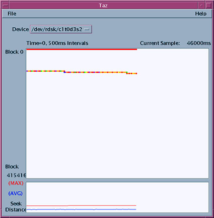
Figure 3. Logging filesystem seeks between log and data

Due to the impact of logging on sequential performance, we can use the Veritas option to mount the filesystem without a log if we're going to create large files. This might be useful when we create database table spaces, or if we require high-performance compute jobs where it's necessary to create large temporary files:

# mount -o nolog /vxfs
# cd /vxfs
# time mkfile 150m 150m

real       32.5
user        0.1
sys        23.6

# iostat -xc 5
device    r/s   w/s   kr/s   kw/s wait actv  svc_t  %w  %b  us sy wt id
fd0       0.0   0.0    0.0    0.0  0.0  0.0    0.0   0   0  15 42  0 43
sd3       0.0   0.0    0.0    0.0  0.0  0.0    0.0   0   0 
ssd0      0.0   0.0    0.0    0.0  0.0  0.0    0.0   0   0 
ssd1      0.0   0.0    0.0    0.0  0.0  0.0    0.0   0   0 
ssd2      0.0   0.0    0.0    0.0  0.0  0.0    0.0   0   0 
ssd3      0.0 100.2    0.0 6400.2  0.0 14.5  144.8   0 100 
ssd4      0.0   0.0    0.0    0.0  0.0  0.0    0.0   0   0

Note the difference in elapsed time -- dropping from four minutes down to 32 seconds. We're also writing much larger clusters than expected. A trace with the Taz utility confirms that the writes to the log device at or near block 0 are no longer done, and as a result we see more concentrated write activity. This is illustrated in Figure 4.

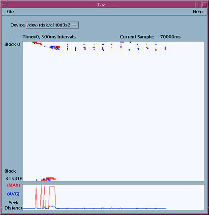
Figure 4. Localized seeking with no logging

Logging in general will have some cost to performance, but there are a wide range of options with each implementation of logging to help overcome some of the performance overhead. Veritas has several levels of logging, ranging from no logging to delayed asynchronous logging to full logging.

UFS, VxFS, and QFS have options that allow metadata to be placed on a disk separate from other data, eliminating the seek patterns we saw in the Taz traces illustrated above. UFS requires that disk suite logging be used to separate log from data. VxFS requires that you purchase the NFS accelerator. QFS does this as an option with the standard QFS filesystem.

Data-intensive random workloads
We can use the truss command to investigate the nature of an application's access pattern by looking at the read, write, and lseek system calls. Below, we use the truss command to trace the system calls generated by our application, processid 19231.

# truss -p 19231

lseek(3, 0x0D780000, SEEK_SET)                  = 0x0D780000
read(3, 0xFFBDF5B0, 8192)                       = 0
lseek(3, 0x0A6D0000, SEEK_SET)                  = 0x0A6D0000
read(3, 0xFFBDF5B0, 8192)                       = 0
lseek(3, 0x0FA58000, SEEK_SET)                  = 0x0FA58000
read(3, 0xFFBDF5B0, 8192)                       = 0
lseek(3, 0x0F79E000, SEEK_SET)                  = 0x0F79E000
read(3, 0xFFBDF5B0, 8192)                       = 0
lseek(3, 0x080E4000, SEEK_SET)                  = 0x080E4000
read(3, 0xFFBDF5B0, 8192)                       = 0
lseek(3, 0x024D4000, SEEK_SET)                  = 0x024D4000

We use the arguments from the read and lseek system calls to determine the size of each I/O and the seek offset at which each read is performed. The lseek system call shows us the offset within the file in hexadecimal. For our example, the first two seeks are to offset 0x0D780000 and 0xA6D0000, or byte numbers 225968128 and 38617088, respectively. These two addresses appear to be random, and further inspection of the remaining offsets show us that the reads are indeed completely random. We can also look at the argument to the read system call and see the size of each read as the third argument. In our example, every read is exactly 8,192 bytes, or 8 KB. In summary, we can see that the seek pattern is completely random, and that the file is being read in 8-KB blocks.

There are several factors that should be considered when configuring a filesystem for random I/O:

Try to match the I/O size and the filesystem block size
Choose an appropriately large filesystem cache
Disable prefetch and read ahead, or limit read ahead to the size of each I/O
Disable filesystem caching when the application does its own caching (e.g., databases)

It is very important to try to match the filesystem block size to a multiple of the I/O size for workloads that include a large proportion of writes. A write to a filesystem that is not a multiple of the block size will result in a partial write of a block. This requires the old block to be read, the new contents to be updated, and the whole block to be written out again. Such a read-modify-write cycle causes a lot of extra I/Os. The I/O size of the application should be chosen to match its block size. Applications that do odd-sized writes should be modified to pad each record out to the nearest possible block size multiple where possible to eliminate the read-modify-write cycle.

Random I/O workload often accesses data in very small blocks (2 KB to 8 KB), and each I/O to and from the storage device requires a seek and an I/O because only one filesystem block is read at a time. Each disk I/O takes on the order of a few milliseconds, and while the I/O is occurring the application needs to stall and wait for it to complete. This can represent a large proportion of the application's response time. As a result, caching filesystem blocks into memory can make a big difference to application performance because we can avoid many of those expensive and slow I/Os. For example, consider a database that does three reads from a storage device to retrieve a customer record from disk. If the database takes 500 microseconds of CPU time to retrieve the record, and spends 3 by 5 milliseconds to read the data from disk, it spends a total of 15.5 milliseconds to retrieve the record -- 97 percent of that time is spent waiting for disk reads.

We can dramatically reduce the amount of time spent waiting for I/Os by caching. We can use memory to cache previously read disk blocks. If that disk block is needed again we simply retrieve it from memory, avoiding the need to go to the storage device again.

I'm not going to get into the particulars of random workloads yet. We'll discuss caching in detail next month.

Summary
So far, we've covered some of the important factors that can affect filesystem performance, and how the filesystem parameters affect performance in different ways.

Next month, we'll examine the Solaris file caching implementation and discuss how the filesystem uses cache and how this, in turn, affects filesystem performance.

Click on our Sponsors to help Support SunWorld

Resources

"Getting to know the Solaris filesystem, Part 1," Richard McDougall (SunWorld, May 1999). Learn all about the inner workings of your on-disk filesystem, including allocation management, storage capacity and access control list support, and metadata logging:
http://www.sunworld.com/swol-05-1999/swol-05-filesystem.html
"RAID: What does it mean to me?" Brian Wong (SunWorld, September 1995). With its cost more reasonable than ever, a redundant array of inexpensive disks (RAID) may be (or perhaps should be) in your future. Here's a primer on the pros and cons of various RAID options:
http://www.sunworld.com/swol-09-1995/swol-09-raid5.html
"What is RAID?" Rawn Shah (Connectivity, SunWorld, June 1999). Rawn Shah clears up a few misconceptions about RAID, one of the most widespread tools for storage management, and gives an idea of what the technology can and can't do for your network:
http://www.sunworld.com/swol-06-1999/swol-06-connectivity.html
"0, 1, 0+1 ... RAID basics," Chuck Musciano (SunWorld, June 1999). Confused about the various RAID configurations and which one is best for your environment? Chuck starts with the basics and explains how RAID 0, 1, and 0+1 function so you can compare characteristics and decide whether or not they fit your network architecture needs:
http://www.sunworld.com/swol-06-1999/swol-06-raid1.html
See Jim Mauro's Inside Solaris columns on Solaris files and ACLs in SunWorld:
http://www.sunworld.com/sunworldonline/common/swol-backissues-columns.html#insidesolaris
See Adrian Cockcroft's Performance Q&A columns in SunWorld:
http://sw/sunworldonline/common/swol-backissues-columns.html#perf
LSC Inc.:
http://www.lsci.com
Veritas Software Corp.:
http://www.veritas.com

Other SunWorld resources

The SunWorld Topical Index -- a comprehensive listing of all SunWorld articles by subject:
http://www.sunworld.com/common/swol-siteindex.html
Visit sunWHERE -- launchpad to hundreds of online resources for Sun users:
http://www.sunworld.com/sunwhere.html
Explore SunWorld's back issues:
http://www.sunworld.com/common/swol-backissues.html
IDG.net, your one-stop IT resource:
http://www.idg.net

About the author
Richard McDougall is an established engineer in the Enterprise Engineering group at Sun Microsystems where he focuses on large system performance and operating system architecture. He has more than 12 years of performance tuning, application/kernel development, and capacity planning experience on many different flavors of Unix. Richard has authored a wide range of papers and tools for measurement, monitoring, tracing and sizing of Unix systems including the memory sizing methodology for Sun, the set of tools known as MemTool allowing fine-grained instrumentation of memory for Solaris, the recent Priority Paging memory algorithms in Solaris and man of the unbundled Tools for Solaris. Richard is currently coauthoring with Jim Mauro the Sun Microsystems book, Solaris Architecture, which details Solaris architecture, implementation, tools, and techniques.

If you have technical problems with this magazine, contact webmaster@sunworld.com

URL: http://www.sunworld.com/swol-06-1999/swol-06-filesystem2.html
Last modified:

Comments:
Name:
Email:
Company Name: